Modelling the Shear Banding in Gradient Nano-Grained Metals
1College of Mechanical and Electrical Engineering, Central South University, Changsha, China
2State Key Laboratory of High Performance Complex Manufacturing, Central South University, Changsha, China
*Corresponding author: mejjli@csu.edu.cn
Nanomaterials 11, 2468 (2021)
Summary
Metals whose grains grow from tens of nanometers at the surface to tens of micrometers inside are both strong and ductile, yet how their nanograined surface deforms has been debated. Nanograined metal on its own fails early through shear bands, narrow zones of concentrated strain, and experiments have found shear bands on the surface of gradient metals even at small strains, where earlier studies had assumed uniform deformation.
This paper models gradient copper with a constitutive law based on dislocation density and a finite element model whose irregular grains, built from Voronoi polygons, grow in size from the surface inward. In the simulations, a shear band forms at the surface at a small strain, as in nanograined copper, but the coarse-grained core stops it, and more bands form as the load grows. The more shear bands form, the larger the uniform elongation, and a smaller grain size distribution index, a thinner gradient layer or larger surface grains give more of them. The model reproduces measured stress–strain curves and shear band patterns, and the paper concludes that gradient metals owe their ductility to shear bands that the gradient keeps stable.
1 Gradient nanograined metals #
In metals, strength usually comes at the cost of ductility. Gradient nanostructures, inspired by materials such as bamboo and shells, offer a way out. In a gradient nanograined metal, the grain size changes gradually from tens of nanometers at the surface to tens of micrometers at the center. In pioneering experiments, gradient nanograined copper made by surface mechanical grinding reached a yield strength of 129 MPa, twice that of coarse-grained copper, while keeping a comparable ductility.
How the nanograined surface layer deforms has remained unclear. On its own, nanograined metal has little ductility and often fails through shear bands that can start at a plastic strain as small as 0.3%. Earlier studies held that the surface layer of a gradient metal deforms uniformly, but closer inspection found shear bands there too. In gradient interstitial-free steel, two shear bands formed at the surface at an applied strain of only 1%; instead of spreading across the sample, they stabilized, and the steel reached a uniform elongation of 20.6%, comparable to its coarse-grained counterpart. Gradient nickel showed dense, dispersed shear bands and still reached a uniform elongation of 30.6%.
This paper builds a computational model to follow how shear bands form and evolve in gradient copper, and how the features of the gradient shape them.
2 Constitutive model #
The model treats gradient copper as a composite: a coarse-grained core under a gradient surface layer, which is split into many thin layers, each with one grain size. Every layer, and the core, follows the same law: elastic deformation by Hooke's law and plastic flow by J2 flow theory, with a flow stress from a modified Kocks–Mecking–Estrin model that Li and coworkers developed for gradient nanostructures. The flow stress adds three terms: the lattice friction, a Taylor hardening term that grows with the density of stored dislocations, and a Hall–Petch term that rises as the grain size falls. The dislocation density evolves with plastic strain through storage and dynamic recovery, with an extra recovery term for nanograins.
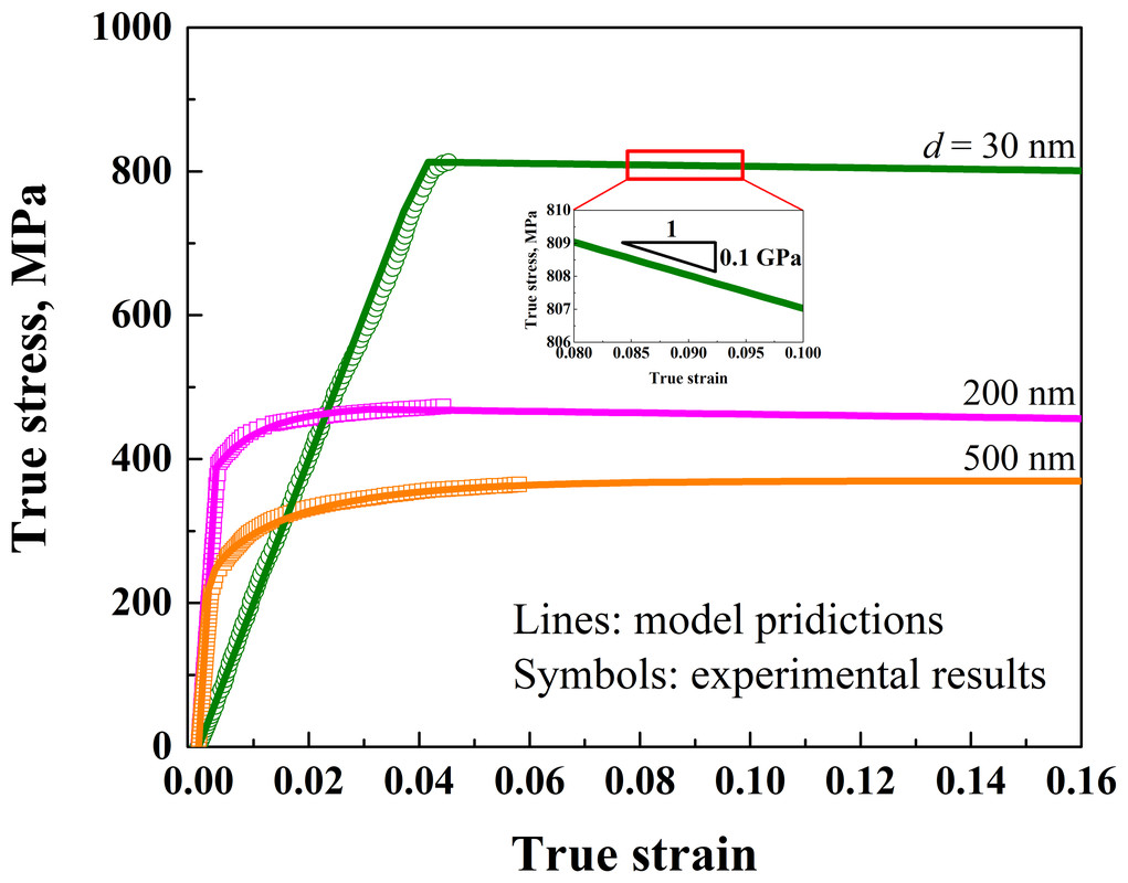
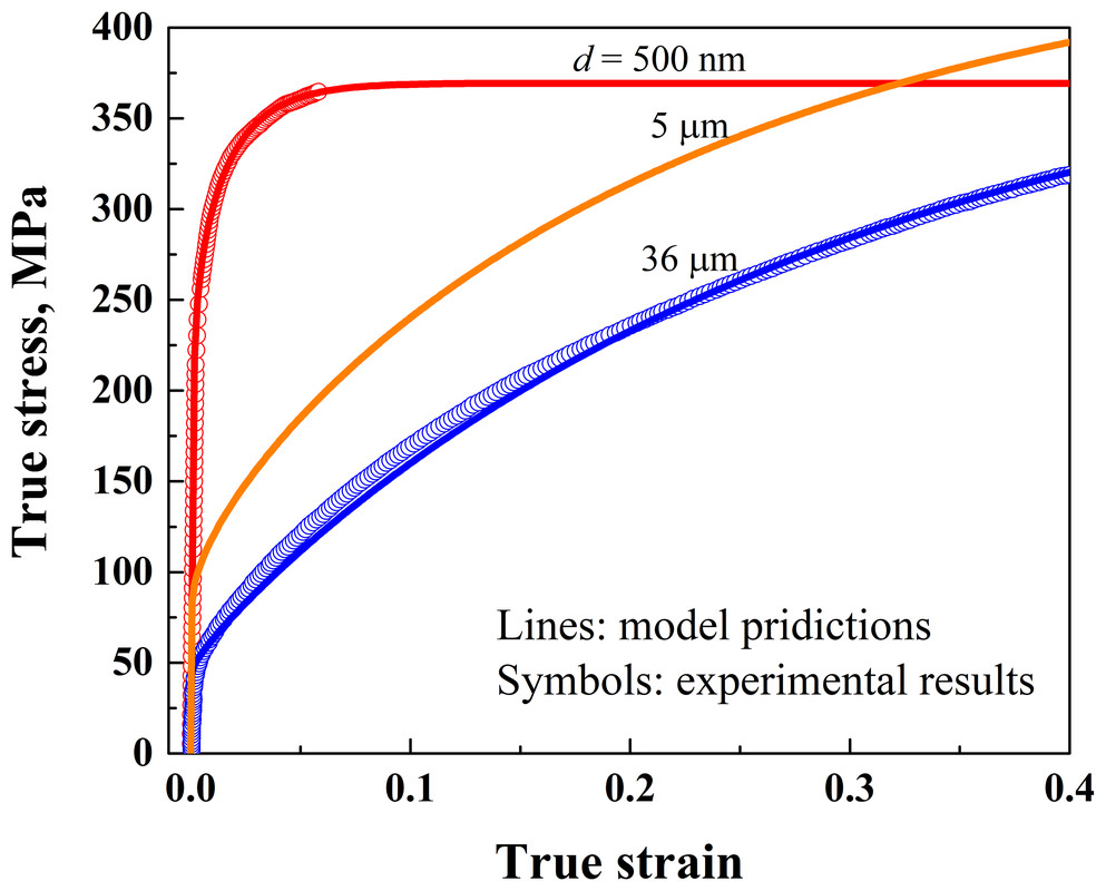
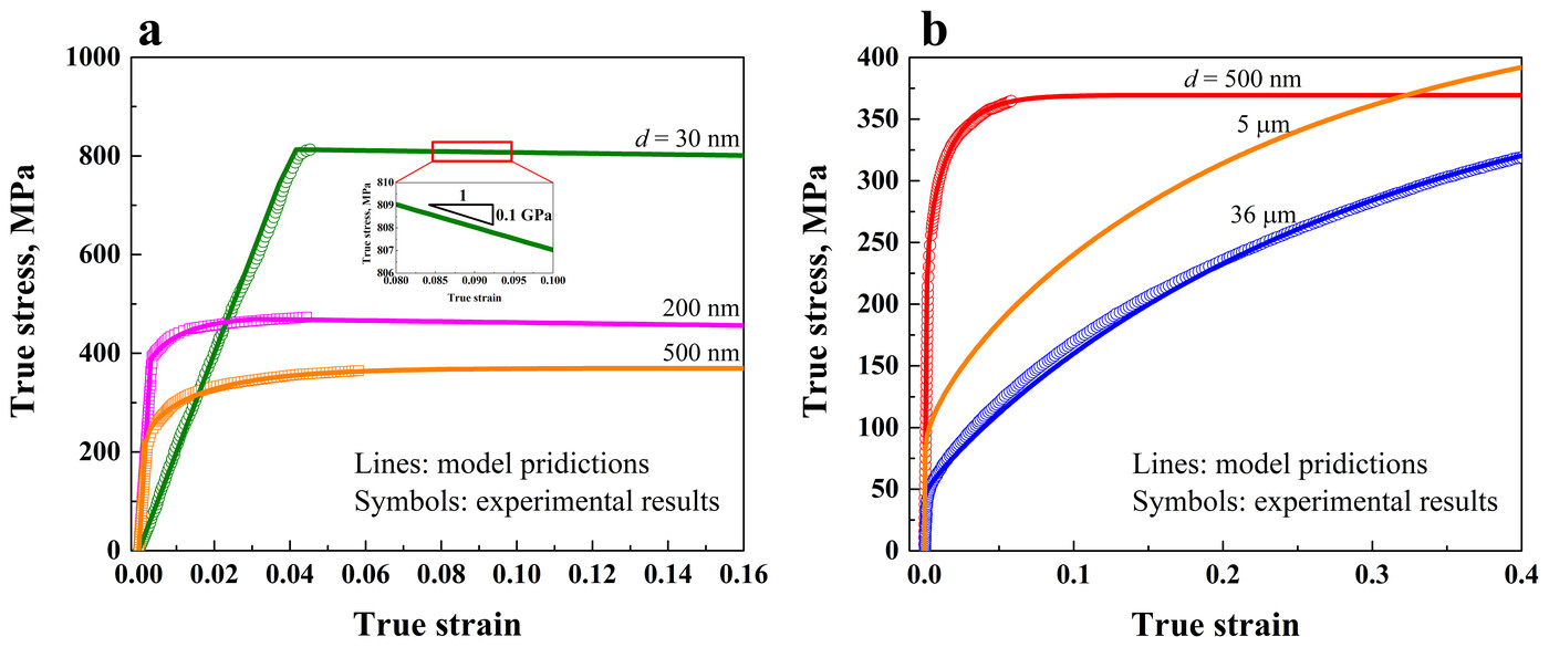
Two sets of parameters cover the grain sizes: one for nanocrystalline grains, below 0.5 µm, and one for microcrystalline grains, from 0.5 to 36 µm. Some come from earlier measurements; the rest were fitted to measured stress–strain curves of copper with 30 nm, 200 nm, 500 nm and 36 µm grains. Because surface treatments leave the nanocrystalline layer with far more dislocations than the untreated core, usually two orders of magnitude more, the nanocrystalline set starts with a dislocation density of 7 × 10¹³ m−2 and the microcrystalline set with none.
Experiments show that the nanograined surface of gradient copper softens as it deforms, so once the nanocrystalline layers pass their uniform elongation, they soften linearly, with a slope of 0.1 GPa, at the low end of the 0.1 to 1 GPa measured for nanocrystalline copper. With these parameters, the model reproduces the measured curves for each grain size.
3 Microstructure and finite element model #
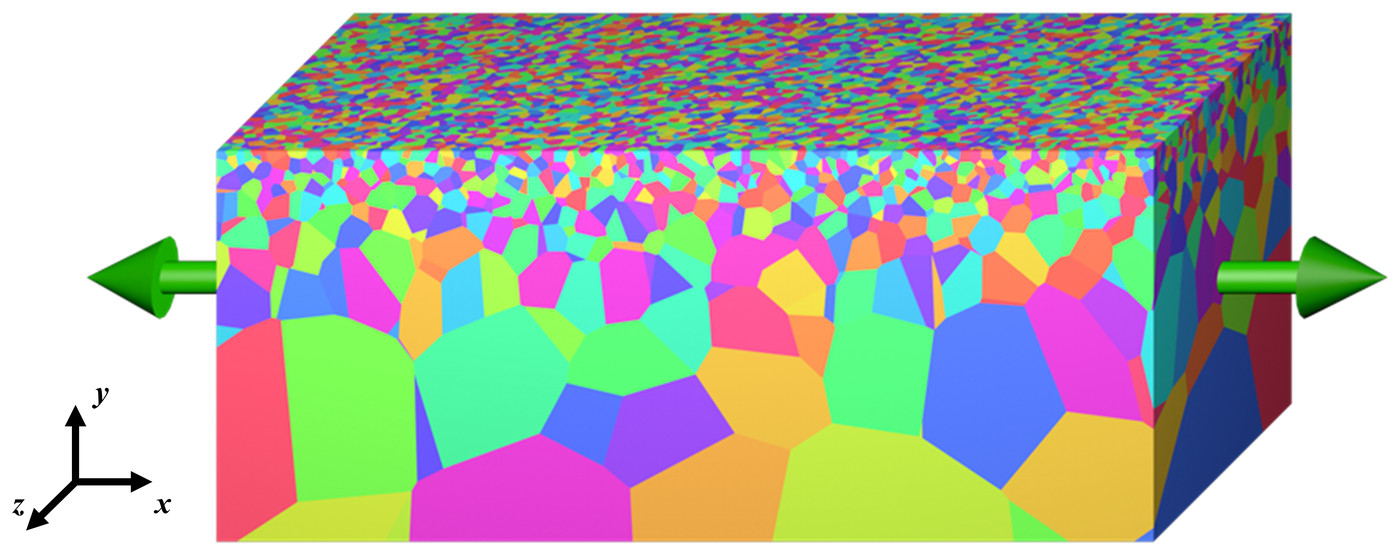
Shear bands tend to form where stress concentrates, and in a gradient metal that is mainly at the boundaries between grains of different sizes. The model therefore builds its grains explicitly, by Voronoi tessellation. Seeds are placed at the centers of ideally arranged grains, one row per layer, then perturbed so that the grain boundaries come out irregular, and the Voronoi cell of each seed becomes a grain.
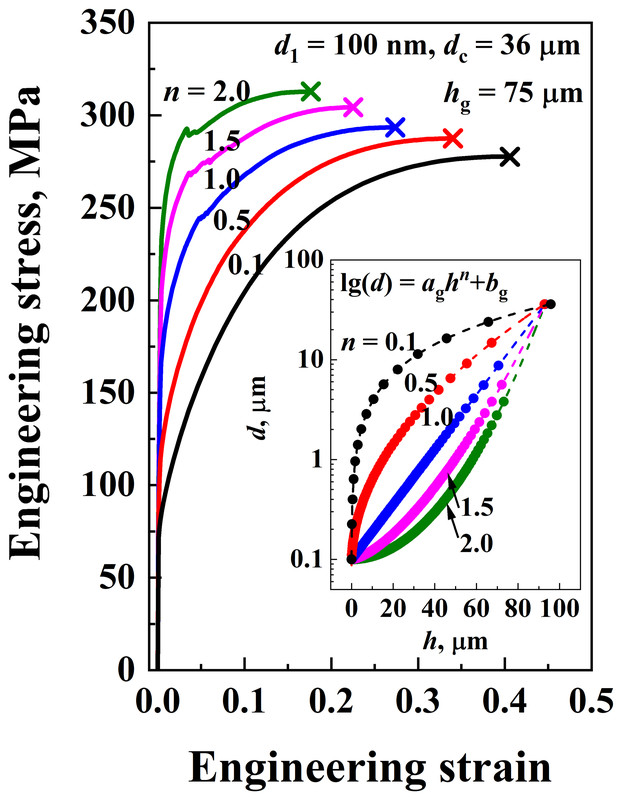
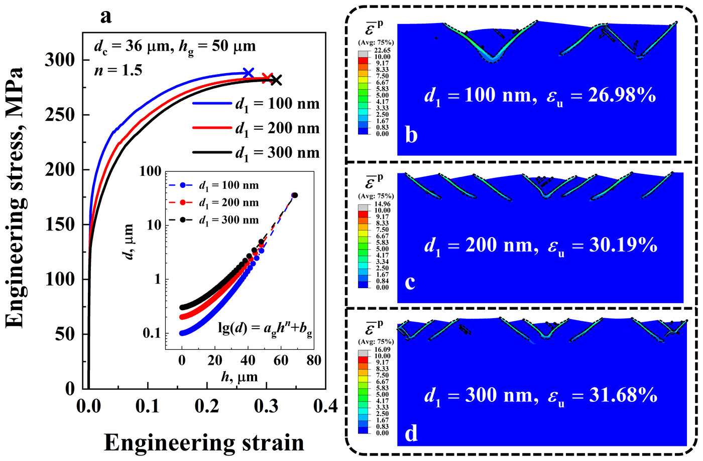
The grain size follows a profile fitted to measurements, lg d = aghn + bg, where h is the depth below the surface, n the grain size distribution index, and ag and bg constants. Each layer is one grain thick, and its grain size is the value of the profile at the middle of the layer. Choosing the surface grain size d1, the core grain size dc, the index n and the number of layers then fixes the constants and the grain size of every layer.
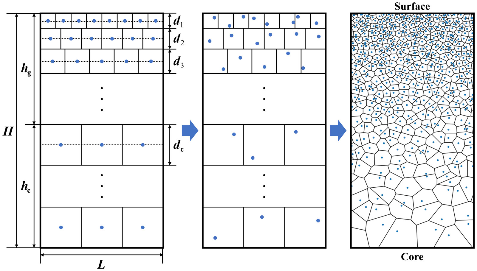
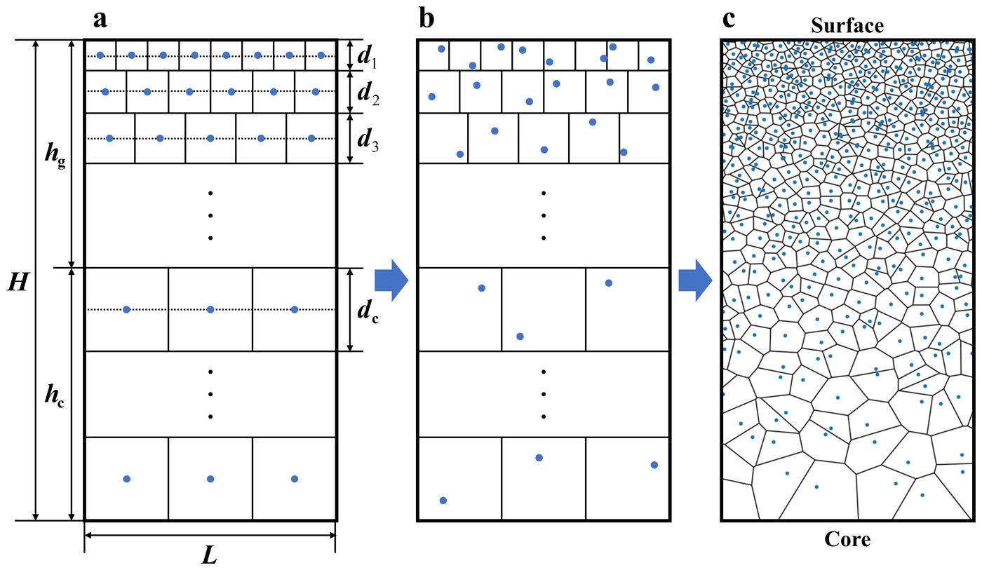
The finite element model keeps only the boundaries between layers of different grain sizes and removes those within each layer, to save computation. The paper's simulations show that this does not change the results, because the boundaries between layers are what induce strain localization and then the shear bands.
The 2D model is 200 µm long and 150 µm thick, with symmetry conditions on its left and bottom edges and a displacement applied to its right edge, and it is meshed in Abaqus with 568,916 four-node and 1308 three-node plane strain elements. Across the 2D simulations, the gradient layer is 25 to 100 µm thick, the surface grains are 100 to 300 nm, the core grains 36 µm, and n ranges from 0.1 to 2. A 3D model, only 4 µm long, 50 µm thick and 1 µm wide because of its cost, with periodic conditions along its length and width, served to check the approach against experiments, below.
4 Shear band multiplication #
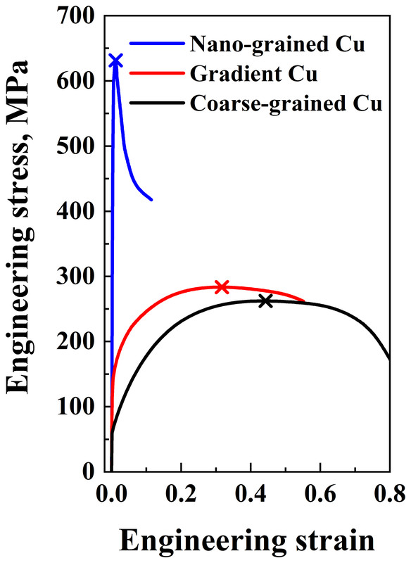
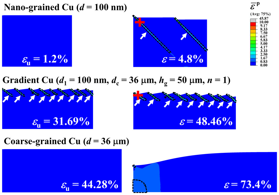
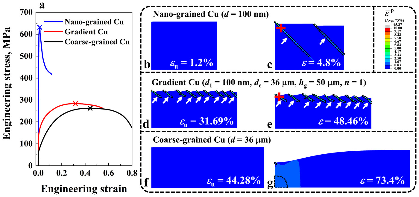
The paper first stretches three models: nanograined copper with 100 nm grains, coarse-grained copper with 36 µm grains, and gradient copper with 100 nm grains at the surface and 36 µm in the core, a 50 µm gradient layer and n = 1. Each has a small notch at its top left corner, 0.5 µm deep and 5 µm wide, to trigger nonuniform deformation in the two uniform materials. The nanograined copper is strong but brittle, with a yield strength of 606.88 MPa and a uniform elongation of 1.2%; the coarse-grained copper is ductile but weak, with 61.81 MPa and 44.28%. The gradient copper combines the two, with a yield strength of 131.68 MPa and a uniform elongation of 31.69%, comparable to that of the coarse-grained copper.
They also deform very differently. In the nanograined copper, two shear bands have already crossed nearly the whole model at an applied strain of 4.8%, which explains its low ductility. The coarse-grained copper deforms without visible localization up to its uniform elongation and then fails by necking. The gradient copper forms many short shear bands along its surface.
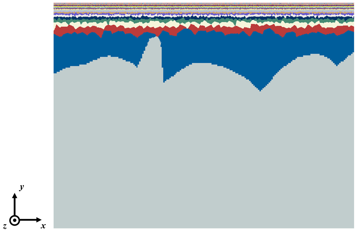
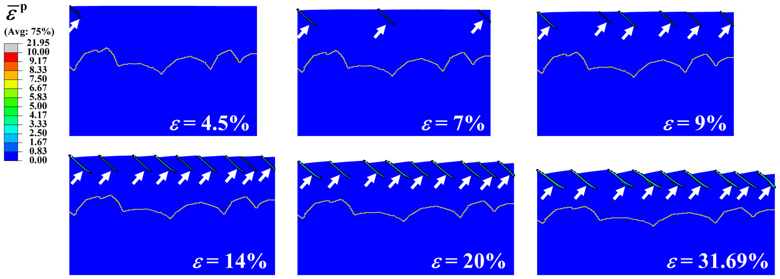
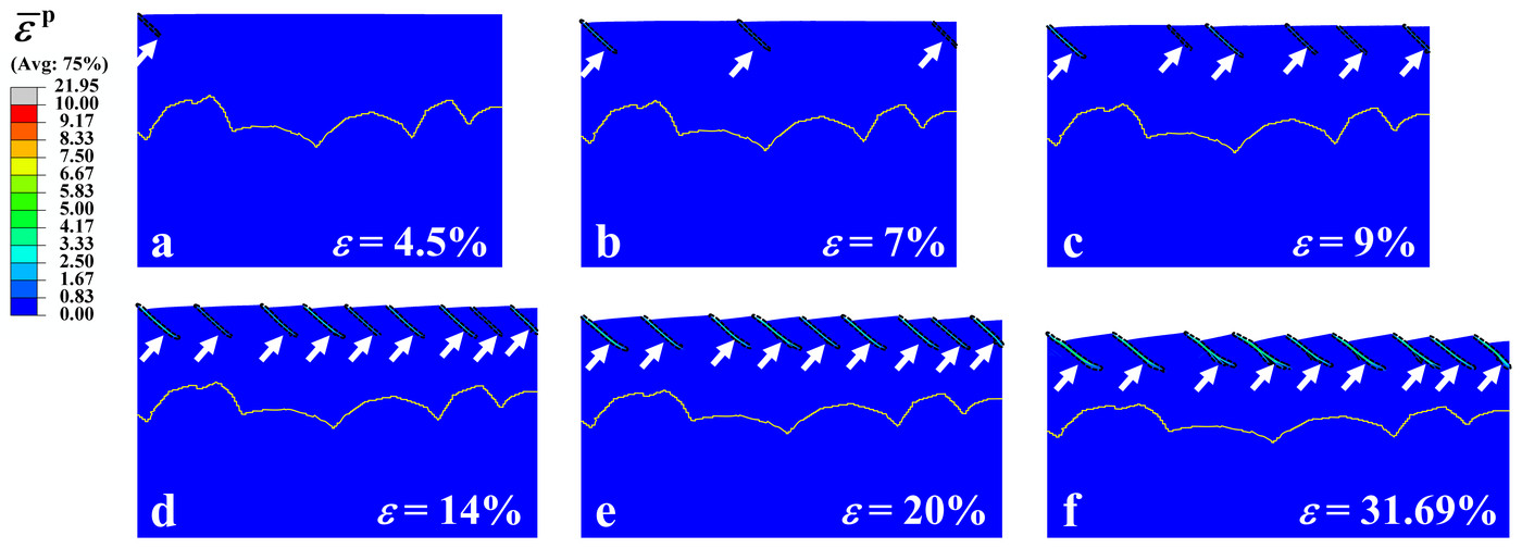
Snapshots of the gradient copper, also shown in the sequence at the top of the page, follow its shear bands. The first band appears at an applied strain of only 4.5%, much as in the nanograined copper and in line with experiments on gradient steel, where a band appeared on the surface at about 1%. But the coarse grains of the core stop it inside the gradient layer, and new bands form instead: from one at 4.5% to six at 9%, until the number levels off at nine after 14%. Experiments on gradient nickel showed the same trend, a density of shear bands that first rises and then stays almost constant.
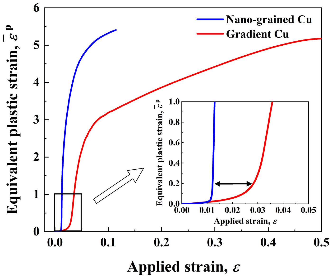
The bands also grow more slowly in the gradient copper. Inside a band, the equivalent plastic strain starts to climb at an applied strain of about 0.012 in the nanograined copper but only at about 0.028 in the gradient copper. Raising it from 1 to 4 then takes an extra applied strain of 0.02 in the nanograined copper and 0.19 in the gradient copper, 9.5 times as much. Stabilized by this multiplication of shear bands, the nanograined surface carries large strains instead of failing early, so the gradient copper gains a high ductility while keeping the strength of its nanograined surface.
5 Effects of the grain size gradient #
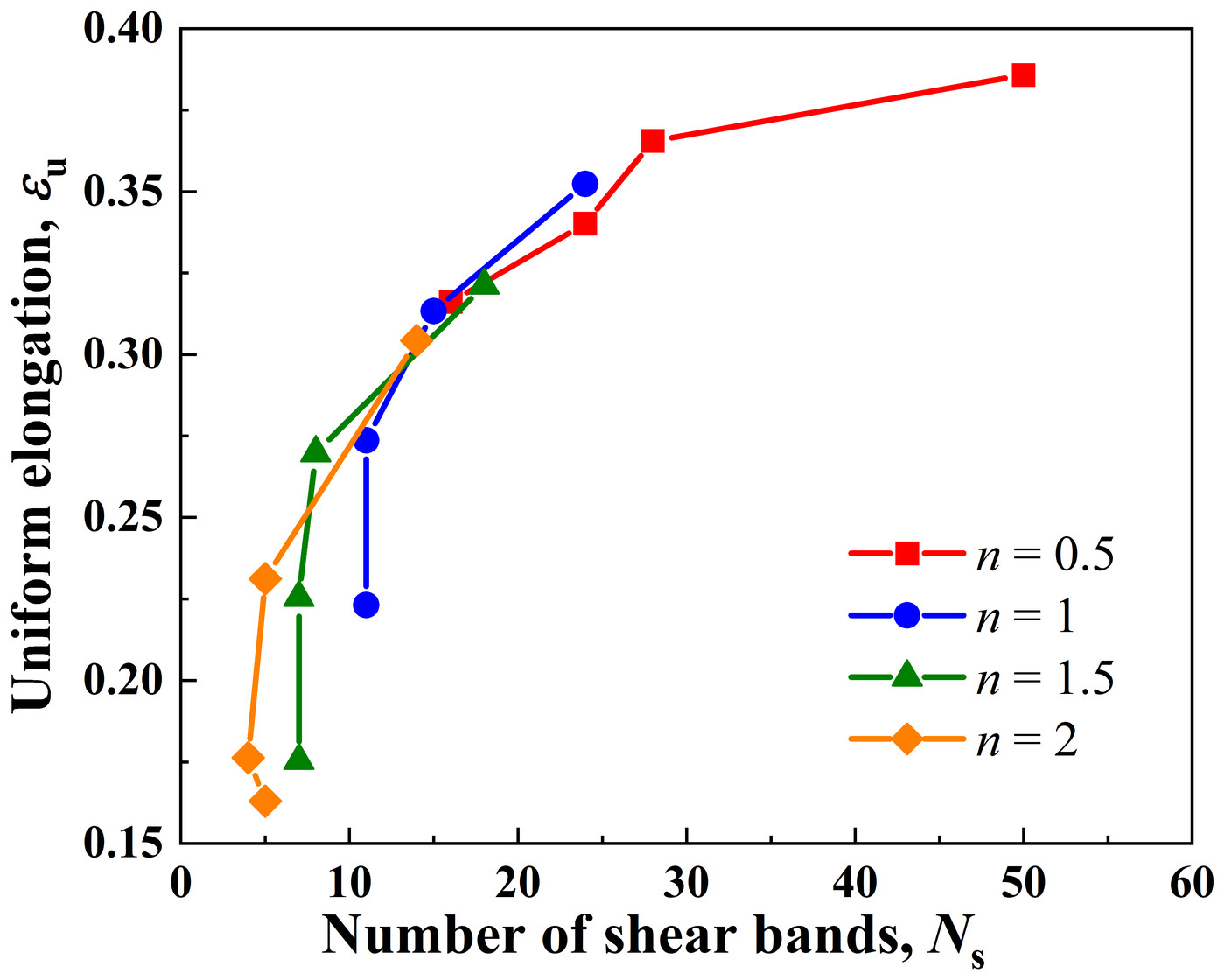
Across the gradients simulated, ductility follows the number of shear bands. With 100 nm grains at the surface, 36 µm grains in the core, n of 0.5, 1, 1.5 and 2 and gradient layers from 25 to 100 µm thick, the uniform elongation rises with the number of shear bands. The most ductile of these cases, with n = 0.5 and a 25 µm layer, formed 50 shear bands and reached a uniform elongation of 38.58%.
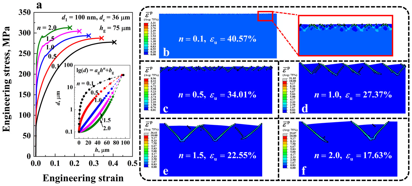
Three features of the gradient set how many bands form, and each trades strength against ductility. A larger index n keeps the grains fine deeper below the surface. With a 75 µm gradient layer, raising n from 0.1 to 2 nearly triples the yield strength, from 79.9 to 222.06 MPa, but more than halves the uniform elongation, from 40.58% to 17.63%. At n = 0.1 a large number of shear bands form along the surface; at n = 2, only three.
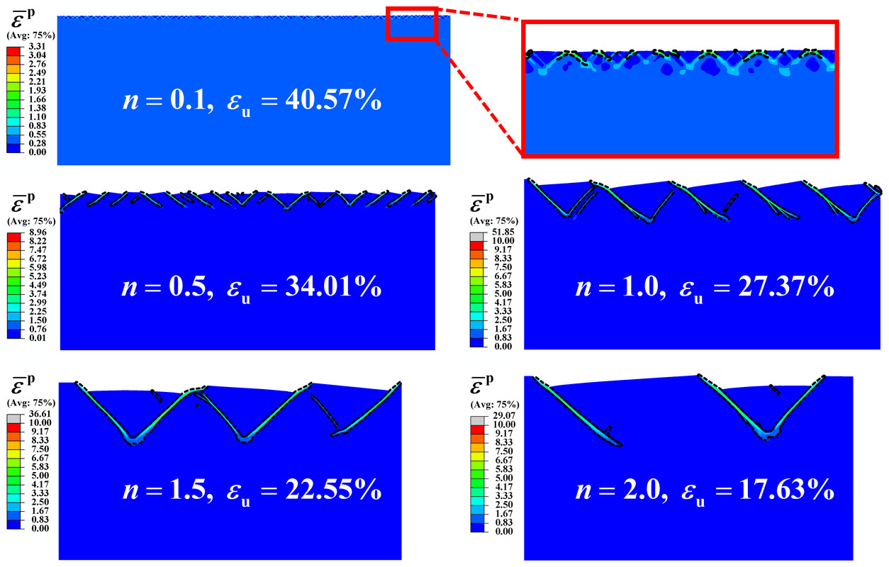
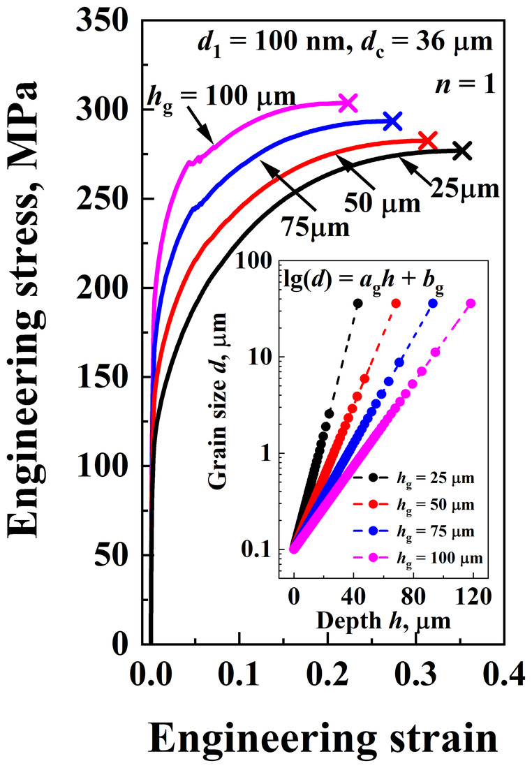
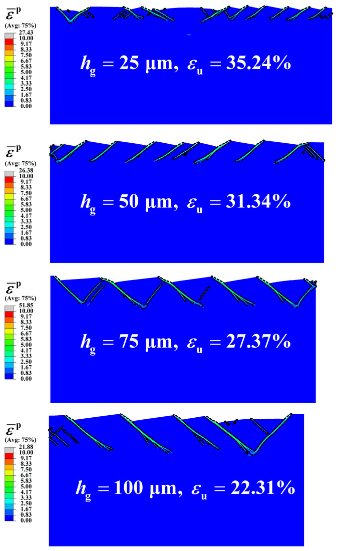
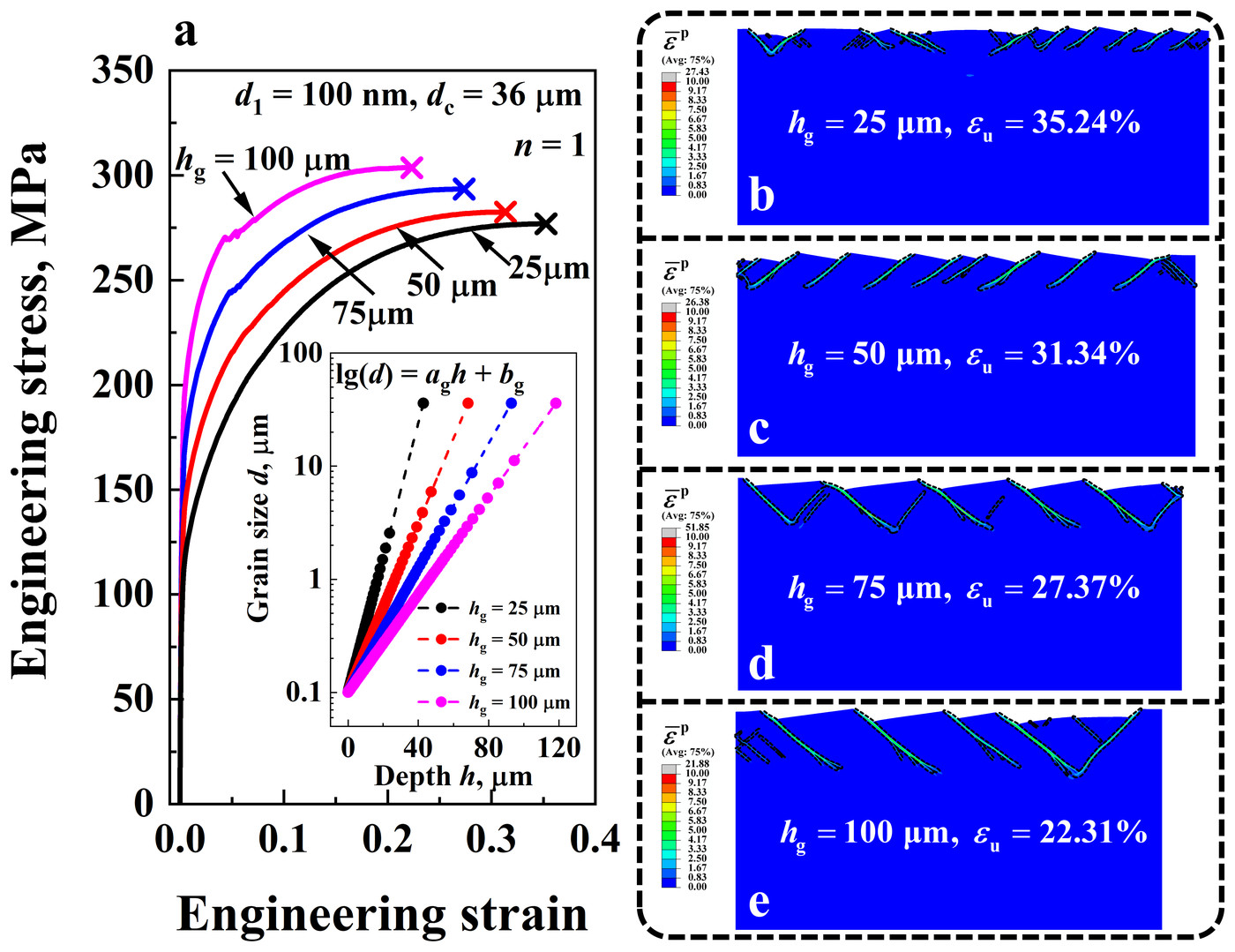
A thicker gradient layer has the same effect. With n = 1, going from a 25 µm to a 100 µm layer raises the yield strength from 106.56 to 187.81 MPa and lowers the uniform elongation from 35.24% to 22.31%; 24 shear bands form with the thin layer and 10 with the thick one.
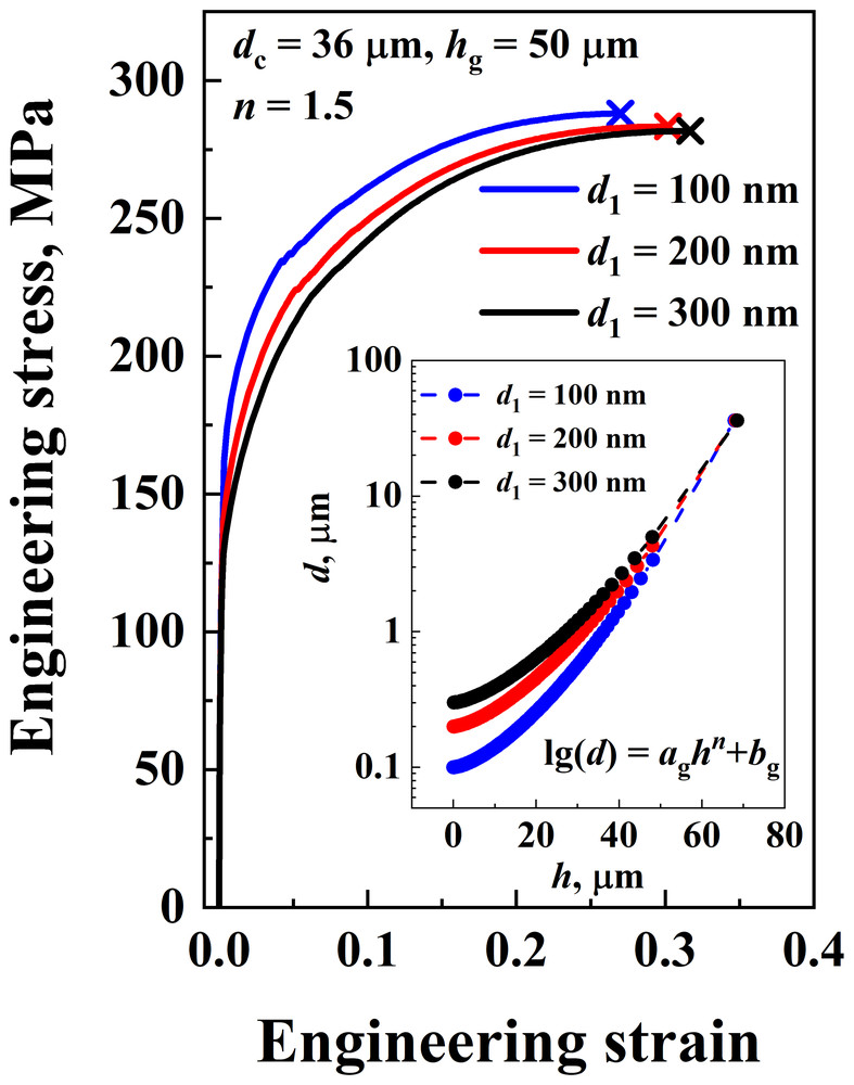
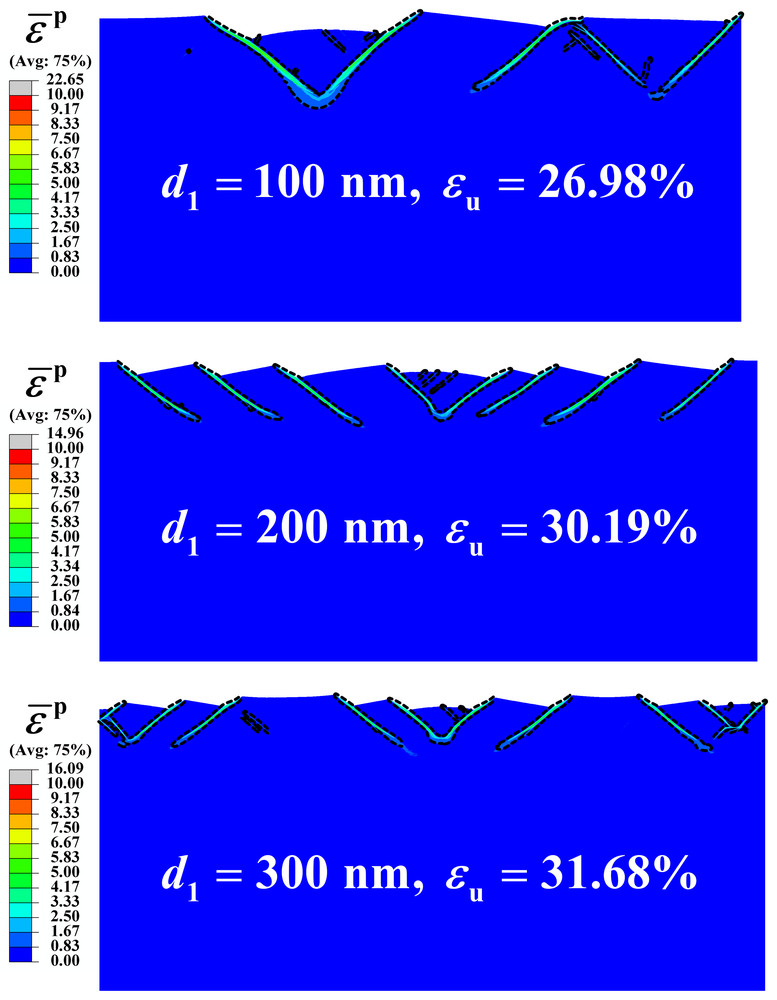
Larger surface grains work the other way. With n = 1.5 and a 50 µm layer, going from 100 to 300 nm grains at the surface lowers the yield strength from 155.65 to 128.2 MPa and raises the uniform elongation from 26.98% to 31.68%, with 13 shear bands instead of 5. In every case, more shear bands spread the plastic strain over more of the nanograined layer, which raises the ductility.
6 Comparison with experiments #
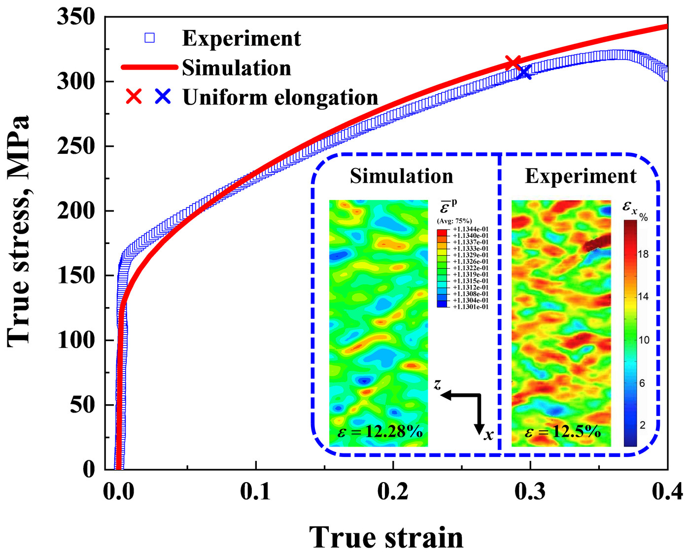
The 3D model checks the approach against tensile tests on gradient copper. With the surface grain size (120 nm), core grain size (36 µm) and volume fraction of the gradient layer (25%) of the tested material, and n = 1.13, the simulated true stress–strain curve follows the measured one: a yield strength of 127.24 MPa and a uniform elongation of 28.73%, against 150.48 MPa and 29.51% measured. The model leaves out fracture, such as the growth of microcracks, so it does not show the drop in stress after uniform elongation.
On the top surface, at an applied strain of about 12.5%, the simulated plastic strain reproduces the shear band pattern of the strain map measured on the sample. The paper finds the model in good agreement with experiments both in the stress–strain response and in how shear bands evolve, including the early bands seen in gradient steel and the band density that levels off in gradient nickel. It notes that strain rate may also affect shear banding in gradient metals, which it leaves for future work.
BibTeX #
@article{chen2021modelling,
  title = {Modelling the Shear Banding in Gradient Nano-Grained Metals},
  author = {Chen, Tianyu and Li, Jianjun},
  journal = {Nanomaterials},
  volume = {11},
  number = {10},
  pages = {2468},
  year = {2021},
  doi = {10.3390/nano11102468}
}